Autofig Basics

autofig aims to provide the following:

a unified calling structure to matplotlib's plot, scatter, errorbar, LineCollection, and PolyCollection in both 2D and 3D projections. So if you decide you want to add errorbars or colorscaling to an existing plot call, you don't need to change the entire calling structure anymore.
unified definition of sizes with multiple options, so resizing a figure doesn't require changing all markersizes/linewidths.
basic "3D" support within 2D figures (by providing the z-coordinate, the z-orders will automatically be set)
a high-level wrapper to animate an existing plot over some independent-variable (i.e. time), with effects including highlight and uncover.
intelligent options for axes limits within animations.
intelligent defaults for subplot creation based on conflicts in units/labels.

import autofig
import numpy as np
import astropy.units as u

Here, depending on your version of Jupyter notebooks, you may need to set inline mode by uncommenting the line below so that the figures show in the notebook (if this doesn't work, you may also need to pass show=True to any autofig.draw() or autofig.animate() calls). In a python script, omit this line, and sending show=True to autofig.draw() or autofig.animate() will popup an interactive matplotlib window.

#autofig.inline()

autofig allows building figures both with a top-down syntax (similar to calling plt.plot(...)) or with an object-oriented bottom-up syntax (similar to fig=plt.figure(); ax=fig.add_subplot(...); ax.plot(...)). To get started, we'll use the top-down approach.

Using the top-down syntax there is really only one main call, autofig.plot. This accepts arrays for each of 6 dimensions (optionally). These dimensions are: * x * y * z (will be used for z-order in 2D plots) * i (the independent variable - either 'x', 'y', 'z' or its own array) * c (color) * s (size)

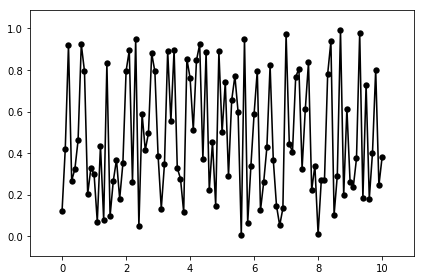
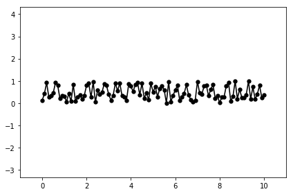
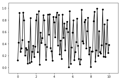
Let's start with a basic plot with just x and y data.

x = np.linspace(0,10,101)
y = np.random.rand(101)

By using the top-down syntax and not creating any objects, autofig will continue to "append" to the existing figure. In order to start over and clear the figure and all previous commands, we'll call autofig.reset. We'll later see other ways to get around this. Passing show=True to the last autofig.plot call or calling autofig.draw() will plot and return the matplotlib figure instance.

autofig.reset()
autofig.plot(x=x, y=y)
mplfig = autofig.draw()

png

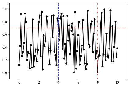
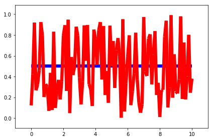
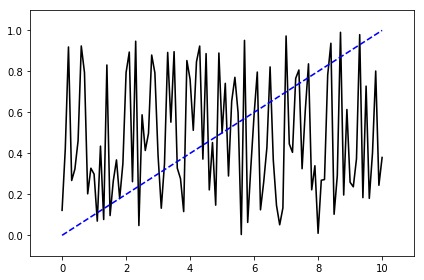
By passing a float instead of an array, a vertical and/or horizontal is drawn:

autofig.reset()
autofig.plot(x=x, y=y)
autofig.plot(x=4)
autofig.plot(x=8, y=0.7)
mplfig = autofig.draw()

png

Labels and Units

In addition, each of the dimensions accept the following optional suffixes: * unit (the units of the provided array, either string or astropy.units object) * error (an array with same length as the values, not accepted for 'c' or 's') * label

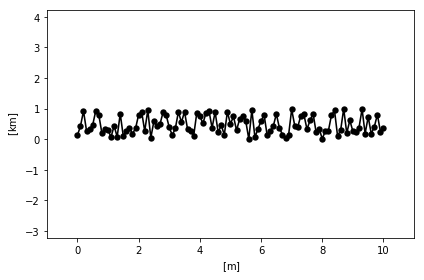
autofig.reset()
autofig.plot(x=x, xlabel='time', xunit=u.s, y=y, ylabel='RV', yunit='km/s')
mplfig = autofig.draw()

png

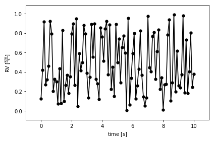
Here we can see that the drawn label is actually the provided label AND the units.

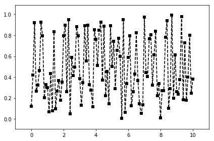
Styling (Markers and Lines)

autofig.plot also accepts the following matplotlib keyword arguments: * marker * linestyle/ls

Note that markersize/ms and linewidth/lw are rejected with an error - these should be sent via the 's' dimension. Similarly, color should be sent via the 'c' dimension.

In each of these cases, if both are provided, the fully spelled-out argument gets priority.

autofig.reset()
autofig.plot(x=x, y=y, marker='s', ls='dashed')
mplfig = autofig.draw()

png

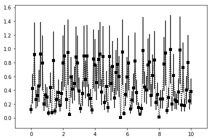
Errorbars

Adding errorbars is as simple as providing an array to the error suffix for a given dimension.

autofig.reset()
autofig.plot(x=x, y=y, yerror=y/2, marker='s', ls='dotted')
mplfig = autofig.draw()

png

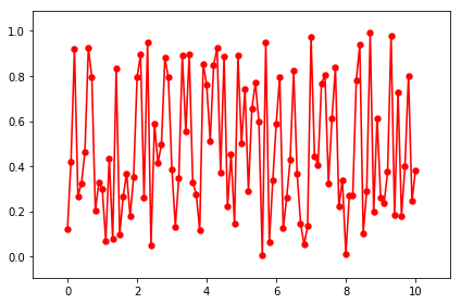
Color

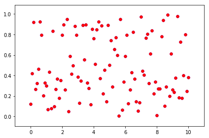
Since 'c' is one of the dimensions, it accepts either an array or a string representing the color to pass on to matplotlib. Note that it affects both the markers and the lines.

autofig.reset()
autofig.plot(x=x, y=y, c='red')
mplfig = autofig.draw()

png

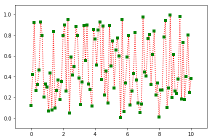
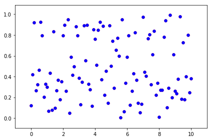
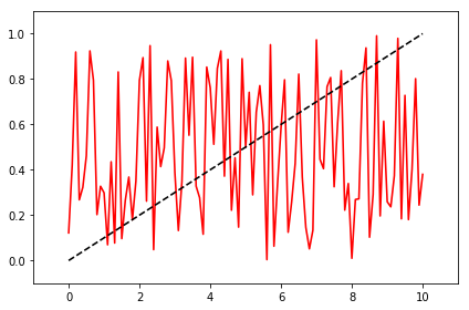
If you want different color treatment for markers and lines you must do so with two separate calls to plot.

autofig.reset()
autofig.plot(x=x, y=y, marker='None', ls='dotted', c='red')
autofig.plot(x=x, y=y, marker='s', ls='None', c='green')
mplfig = autofig.draw()

png

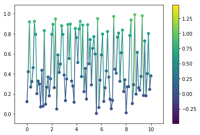
Now let's pass an array to the color dimension, as it is a dimension it also accepts label and unit.

c = y**2

autofig.reset()
autofig.plot(x=x, y=y, 
             c=c, clabel='temp', cunit=u.K, cmap='afmhot')
mplfig = autofig.draw()

png

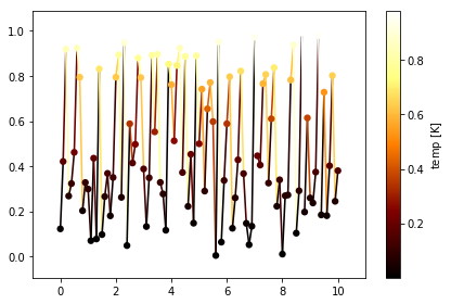
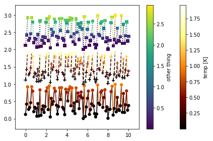
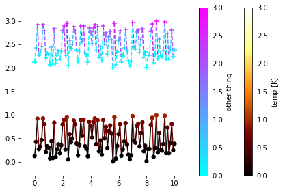
Colorscales and colorbars will be shared (per-axes) whenever there is no conflict between the 'c' dimension's label, units, and colormap.

autofig.reset()
autofig.plot(x=x, y=y, c=c, clabel='temp', cunit=u.K, cmap='afmhot')
autofig.plot(x=x, y=y+1, c=2*c, clabel='temp', cunit=u.K, cmap='afmhot')
autofig.plot(x=x, y=y+2, c=3*c, clabel='other thing')
mplfig = autofig.draw()

png

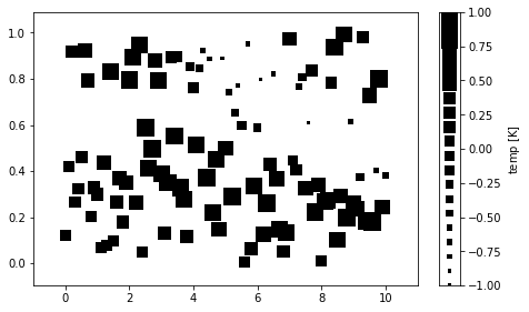
Size

Since 's' is also a dimension, it accepts either an array or float represent the markersizes and linewidths in units of the axes-size (i.e. 0.01 will takeup approximately 1% of the axes). See the size-mode tutorial for more details and other available "modes" for size-scaling.

autofig.reset()
autofig.plot(x=x, y=y, s=0.02)
mplfig = autofig.draw()

png

s = np.sin(x*y)

autofig.reset()
autofig.plot(x=x, y=y,
             s=s, slabel='temp', sunit='K', 
             marker='s', ls='None')
mplfig = autofig.draw()

png

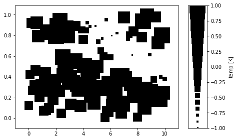
Similarly to cmap, when scaling by size you can pass a tuple to smap. This tuple will give the lower and upper bounds of the point sizes that the entire range will be mapped onto. By default this is (0.01,0.05), but if we want a smaller range of sizes, for example, we could do the following:

s = np.sin(x*y)

autofig.reset()
autofig.plot(x=x, y=y,
             s=s, slabel='temp', sunit='K', smap=(0.01,0.1),
             marker='s', ls='None')
mplfig = autofig.draw()

png

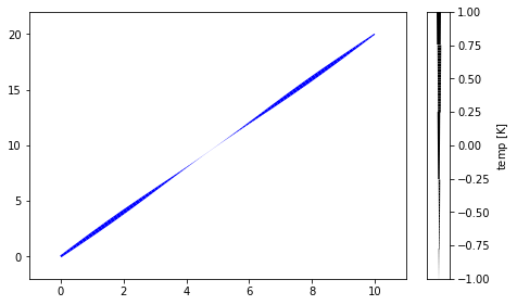
We can also have the size dimension handle linewidths:

s = np.sin(x)

autofig.reset()
autofig.plot(x=x, y=2*x,
             s=s, slabel='temp', sunit='K', smap=(0.001, 0.05),
             c='blue', marker='None', ls='solid')
mplfig = autofig.draw()

png

Limits and Padding

As can be seen above, by default axes limits are set to encompass all of the data (ignoring the hidden data if uncover=True) and accounting for default padding.

See the limits tutorial for a full explanation of all the various options for limits and their influence on animations.

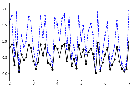
In short, limits can be passed directly to the plot command. If multiple limits are passed to the same axes, the last value will take priority.

autofig.reset()
autofig.plot(x=x, y=y, xlim=(0,20))
autofig.plot(x=x, y=y*2, xlim=(2, 7))
mplfig = autofig.draw()

png

When setting manual limits, padding is ignored. However, we can also send a value for padding directly through the plot command. As per-limits, the last value takes priority.

By default, padding is set to 10% for cartesian (x, y, z) dimensions and 0% for color and size.

autofig.reset()
autofig.plot(x=x, y=y, xpad=0.5)
mplfig = autofig.draw()

png

Limits and padding are available for each of the dimensions (except 'i'). However, in addition to the single dimensions, there are a few "groups" in which you can set multiple settings simultaneously:

xy (xylim, xypad)
xyz (xyzlim, xyzpad)
cs (all currently-existing colorscales; cslim, cspad)
ss (all currently-existing sizescales; sslim, sspad)

Be careful if passing values to both a group and a single dimension - the order to which they are applied may be random. For example, avoid passing xlim and xylim in the same call.

autofig.reset()
autofig.plot(x=x, y=y, xypad=0.5)
mplfig = autofig.draw()

png

autofig.reset()
autofig.plot(x=x, y=y, c=c, cpad=0.5)
mplfig = autofig.draw()

png

autofig.reset()
autofig.plot(x=x, y=y, c=c, clabel='temp', cunit=u.K, cmap='afmhot')
autofig.plot(x=x, y=y+2, c=3*c, clabel='other thing', cmap='cool', cslim=(0,3))
mplfig = autofig.draw()

png

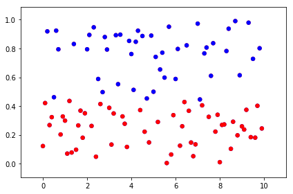
Z-Order

The 'z-order' at which the plotting calls are drawn from back-to-front are according to their z-dimensions. If a single value is given for z, that will be applied to all points, otherwise the z-order is determined on a per-point basis.

For any z not provided, that call's z-order will default to z=-infinity. All plots with z=-infinity will then be drawn in the order they were called.

autofig.reset()
autofig.plot(x=x, y=y, z=10, c='red', marker='o', linestyle='none')
autofig.plot(x=x, y=y, z=5, c='blue', marker='o', linestyle='none')
mplfig = autofig.draw()

png

autofig.reset()
autofig.plot(x=x, y=y, z=5, c='red', marker='o', linestyle='none')
autofig.plot(x=x, y=y, z=10, c='blue', marker='o', linestyle='none')
mplfig = autofig.draw()

png

autofig.reset()
autofig.plot(x=x, y=y, z=y, c='red', marker='o', linestyle='none')
autofig.plot(x=x, y=y, z=-4+10*y, c='blue', marker='o', linestyle='none')
mplfig = autofig.draw()

png

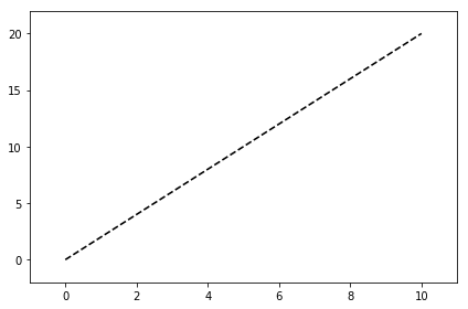
NOTE: when any given segment of a line is small, using a linestyle other than 'solid' is hard to see.

autofig.reset()
autofig.plot(x=x, y=2*x, linestyle='dashed', marker='none')
mplfig = autofig.draw()

png

autofig.reset()
autofig.plot(x=x, y=2*x, z=2*x, linestyle='dashed', marker='none')
mplfig = autofig.draw()

png

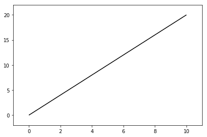
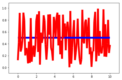
NOTE: the z-order of each segment of the line is determined based on the point to the left. In the future interpolation within the segment may be supported (but then non-solid lines will never show). We can see this below. The first case blue changes its order wrt red throughout the plot, whereas in the second case blue is always below red because the entire segment is getting its zorder from the left point.

autofig.reset()
autofig.plot(x=x, y=y, z=x, linestyle='solid', marker='none', color='r', s=0.08)
autofig.plot(x=x, y=0*y+0.5, z=-5+2*x, linestyle='solid', marker='none', color='b', s=0.08)
mplfig = autofig.draw()

png

autofig.reset()
inds = [0, -1]
autofig.plot(x=x, y=y, z=x, 
             linestyle='solid', marker='none', 
             color='r', s=0.08)
autofig.plot(x=x[inds], y=0*y[inds]+0.5, z=-5+2*x[inds], 
             linestyle='solid', marker='none', 
             color='b', s=0.08)
mplfig = autofig.draw()

png

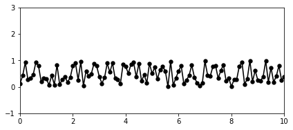
Aspect Ratio

By default, if both x and y dimensions are of the same physical type, then equal aspect ratio will be used. To override this default, you can set 'equal_aspect' to True or False.

If axes limits are not explicity provided, then the axes limits will be adjusted to pad. If axes limits are explicitly provided, then the size of the axes itself will be adjusted to maintain an equal aspect ratio. To override this default, you can set 'pad_aspect' to True or False.

autofig.reset()
autofig.plot(x=x, y=y)
mplfig = autofig.draw()

png

autofig.reset()
autofig.plot(x=x, y=y, equal_aspect=True)
mplfig = autofig.draw()

png

autofig.reset()
autofig.plot(x=x, y=y, equal_aspect=True, xlim=(0,10), ylim=(-1,3))
mplfig = autofig.draw()

png

autofig.reset()
autofig.plot(x=x, y=y, equal_aspect=True, pad_aspect=True, xlim=(0,10), ylim=(-1,3))
mplfig = autofig.draw()

png

NOTE: this means that 'km' vs 'm' will have an equal aspect ratio, but currently ignores the unit itself. This behavior may be changed in the future.

autofig.reset()
autofig.plot(x=x, y=y, xunit='m', yunit='km')
mplfig = autofig.draw()

png

Property Cycler

As you may have noticed, autofig attempts to set reasonable defaults for all properties (color, linestyle, marker, etc) when no value is provided (or None is sent).

Sending None to linestyle or marker will fallback on the defaults (provided by the property cycler), whereas the strings 'None' or 'none' will result in no line or marker drawn, respectively.

autofig.reset()
autofig.plot(x=x, y=y, linestyle=None)
mplfig = autofig.draw()

png

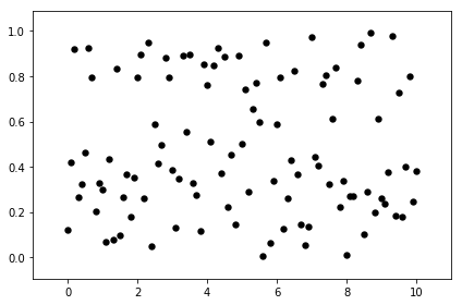
autofig.reset()
autofig.plot(x=x, y=y, linestyle='None')
mplfig = autofig.draw()

png

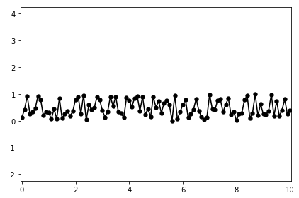
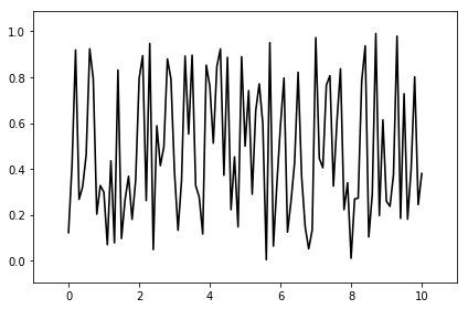
When multiple calls are made, Nones are replaced with the next available entry from the cycler, which is handled on a per-axes (not per-figure) basis.

autofig.reset()
autofig.plot(x=x, y=y, marker='None')
autofig.plot(x=x, y=0.1*x, marker='None')
mplfig = autofig.draw()

png

In the case above, where no color or linestyle were provided for either call to plot, both followed the order of their respective cyclers (black -> blue for color and solid -> dashed for linestyle).

If we set the color on the first call to be red, the second will default to black since it is unused.

autofig.reset()
autofig.plot(x=x, y=y, marker='None', c='red')
autofig.plot(x=x, y=0.1*x, marker='None')
mplfig = autofig.draw()

png

And lastly, by setting the second to black the first will need to change to the second color in the cycler. Note that it originally starts as black, but since the color is set to None, it will change when the second call is added.

autofig.reset()
autofig.plot(x=x, y=y, marker='None')
mplfig = autofig.draw()

png

autofig.plot(x=x, y=0.1*x, marker='None', color='k')
mplfig = autofig.draw()

Independent Variable

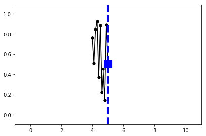
By defining the independent variable, we can draw our figure at a given value of that variable.

autofig.reset()
autofig.plot(x=x, y=y, i='x')
mplfig = autofig.draw(i=5)

png

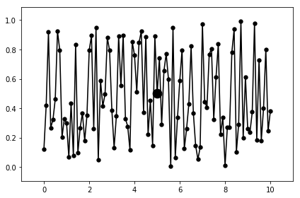
Here we can see a blue dot drawn highlighting the value at i=5.

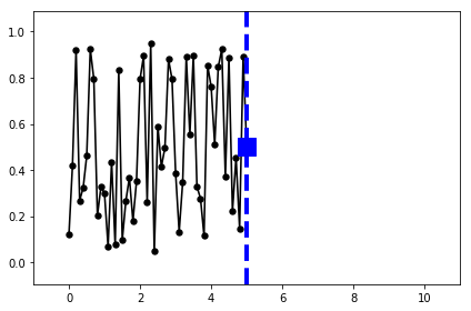
There are several available effects for the independent variable which accept the corresponding additional arguments: * highlight (True/False) * highlight_marker (defaults to 'o') * highlight_color (defaults to color) * highlight_size (defaults to size) * highlight_linestyle (defaults to 'None') * uncover (True/False) * trail (True/False/float representing % in i)

autofig.reset()
autofig.plot(x=x, y=y, i='x', 
             uncover=True,
             highlight=True, 
             highlight_color='b', 
             highlight_marker='s', 
             highlight_size=0.05, 
             highlight_linestyle='dashed')
mplfig = autofig.draw(i=5)

png

autofig.reset()
autofig.plot(x=x, y=y, i='x', 
             uncover=True,
             highlight=True, 
             highlight_color='b', 
             highlight_marker='s', 
             highlight_size=0.05, 
             highlight_linestyle='dashed',
             trail=0.1)
mplfig = autofig.draw(i=5)

png

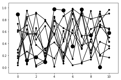
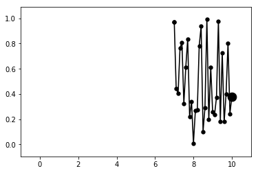
Selecting on Independent Variable

indeps = np.linspace(0,10,11)
xs = [np.linspace(0,10,11) for i in indeps]
ys = [np.random.rand(11) for i in indeps]

autofig.reset()
autofig.plot(x=xs, y=ys, i=indeps)
mplfig = autofig.draw()

png

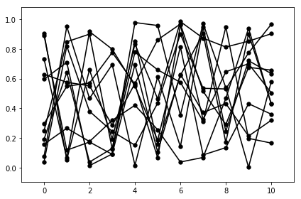
autofig.reset()
autofig.plot(x=xs, y=ys, i=indeps)
mplfig = autofig.draw(i=3)

png

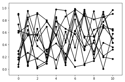
autofig.reset()
autofig.plot(x=xs, y=ys, i=indeps, show=True, uncover=True)
mplfig = autofig.draw(i=3)

png

autofig.reset()
autofig.plot(x=xs, y=ys, i=indeps, show=True, uncover=True, trail=0)
mplfig = autofig.draw(i=3)

png

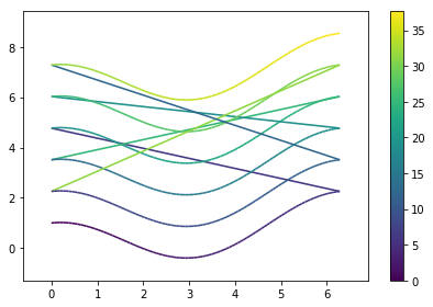
Sorting by Independent Variable

order = [1,4,3,5,2,6]
t_indep = np.concatenate([np.linspace((i-1)*2*np.pi, i*2*np.pi, 100) for i in order])
x_indep = np.concatenate([np.linspace(0, 2*np.pi, 100) for i in order])
y_indep = np.cos(x_indep)+t_indep/5

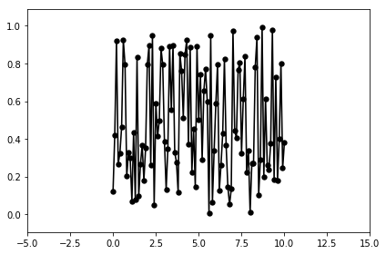
When i is not provided, the plots will be drawn in the order of the arrays provided.

autofig.reset()

autofig.plot(x_indep, y_indep, c=t_indep, marker='None')
mplfig = autofig.draw()

png

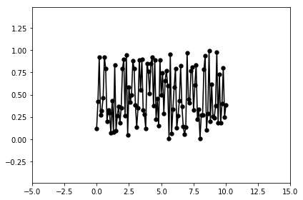
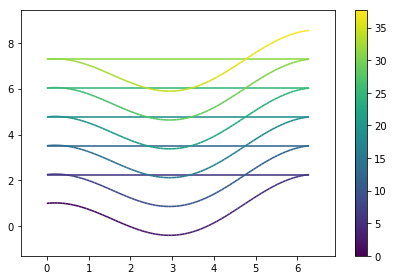
However, when providing i, the points will be re-sorted in increasing i (this is only really noticeable when linestyle is enabled)

autofig.reset()
autofig.plot(x_indep, y_indep, i=t_indep, c=t_indep, marker='None')
mplfig = autofig.draw()

png

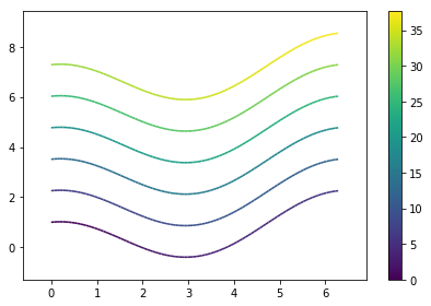
To avoid the line drawing when decreasing in x, pass linebreak='x-' (meaning the line won't be drawn whenever x is decreasing). The value to linebreak can be None (don't break lines, which is the default), or '<+/->' where direction is one of the dimensions in the call (i.e. x, y, z, i, c, s) followed by a '+' (for increasing) or '-' (for decreasing).

autofig.reset()
autofig.plot(x_indep, y_indep, i=t_indep, c=t_indep, marker='None', linebreak='x-')
mplfig = autofig.draw()

png

Animations

Creating an animation is as simple as calling animate instead of draw and passing a list of values to loop over for the independent variable (interpolation will be used, so they don't need to be a member of the original data array).

autofig.reset()
autofig.plot(x=x, y=y, i='x', uncover=True, trail=0.3)
anim = autofig.animate(i=np.linspace(0,10,201),
                       save='basics_x.gif', save_kwargs={'writer': 'imagemagick'})

png

animation

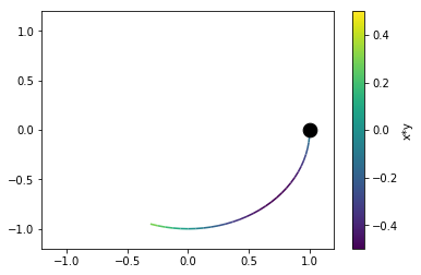
In some cases the independent variable may not be one of the plotted dimensions (time, for example).

t = np.linspace(0, 2*np.pi, 101)
x = np.cos(t)
y = np.sin(t)
c = x*y

autofig.reset()
autofig.plot(x=x, y=y, i=t, c=c, clabel='x*y',
             marker='None', uncover=True, trail=0.3)
anim = autofig.animate(i=t, 
                       save='basics_i.gif', save_kwargs={'writer': 'imagemagick'})

png

animation

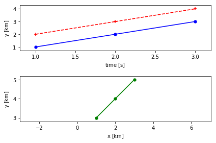
Subplots

When making calls to plot, autofig determines whether that call is consistent with any of the existing axes/subplots. If not, it creates a new one and handles the subplot grid accordingly.

A plot is inconsistent with an existing axes if any of the following conditions is True:

non-identical label in any cartesian or independent-variable (x,y,z,i) dimension (with None or omitted labels ignored)
non-identical title (axes title) (with None or omitted titles ignored)
inconsistent (different physical type) units in any cartesian or independent-variable (x,y,z,i) dimension (None or omitted is assumed to be unitless and can therefore cause inconsistency)

For more information on creating custom layouts see the subplot/axes positioning documentation.

autofig.reset()
autofig.plot(x=[1,2,3], xunit='s', xlabel='time',
             y=[1,2,3], yunit='km', ylabel='y',
             color='blue')
autofig.plot(x=[1,2,3], xunit='s',
             y=[2,3,4], yunit='km',
             color='red')
autofig.plot(x=[1,2,3], xunit='km', xlabel='x',
             y=[3,4,5], yunit='km', ylabel='y',
             color='green')
mplfig = autofig.draw()

png